Fractals
Chaos and Time-Series Analysis
11/14/00 Lecture #11 in Physics 505
 Comments on Homework
#9 (Autocorrelation Function)
-
There was a certain confusion about the notation
-
The autocorrelation function of Lorenz is ~ 6 x 0.05 = 0.3 seconds

 Review (last
week) - Nonlinear Prediction and Noise Reduction
-
Autocorrelation Function
-
g(n) = S (Xi
- Xav)(Xi+n - Xav)
/ S (Xi - Xav)2
-
Correlation time is width of g(n) function (call it
tau)
-
tau can be taken as the value of n for which g(n)
= 1/e = 37%
-
0.5/tau is sometimes called a "poor-man's Lyapunov exponent"
-
From the correlation function g(n), the power spectrumP(f)
can be found:
P(f) = 2 S g(n)
cos(2pfnDt)
Dt
(ref: Tsonis)
-
Time-Delayed Embeddings
-
(Almost) any variable(s) can be analyzed
-
Create multi-dimensional data by taking time lags
-
May need up to 2m + 1 time lags to avoid intersections
where m is the dimension of solution manifold
-
Must choose an appropriate DE (embedding dimension)
-
Increase DE until topology of attractor (dimension)
stops
changing
-
Or use the method of false nearest neighbors
-
Must choose an appropriate Dt
for sampling a flow
-
Summary of Important Dimensions
-
Configuration (or state) space (number of independent dynamical
variables)
-
Solution manifold (the space in which the solution "lives" - an
integer)
-
Attractor dimension (fractional if it's a strange attractor)
-
Kaplan-Yorke (Lyapunov) dimension
-
Hausdorff dimension
-
Cover dimension
-
Similarity dimension (see below)
-
Capacity dimension (see below)
-
Information dimension
-
Correlation dimension (next week)
-
... (infinitely many more)
-
Observable (1-D for a univariate (scalar) time series: Xi)
-
Reconstructed (time-delayed) state space (can be chosen arbitrarily)
-
Time-delayed embedding (the minimum time-delayed state space that
preserves the topology of the solution)
 Nonlinear Prediction
-
There are many forecasting (prediction) methods
-
Conventional linear prediction methods apply in the time domain
-
Fit the data to some function of time and evaluate it
-
The function of time may be nonlinear
-
The dynamics are usually assumed to be linear
-
Linear equations can have oscillatory or exponential solutions
-
Nonlinear methods usually apply in state space
-
Example (predicting next term in Hénon map - HW #
11):
-
We know Xn+1 = 1 - CXn2
+ BXn-1
-
In a 2-D embedding, the next value is unique

-
Find M nearest points in Xn-Xn-1
space
-
Calculate their average displacement: DX
= <Xn+1 - Xn>
-
Use DX to predict next value in
time series
-
Repeat as necessary to get future time steps
-
Sensitive dependence will eventually spoil the method
-
Method does not necessary keep you on the attractor (but could be
modified to do so)
-
Growth of prediction error crudely gives the Lyapunov exponent
-
Example (Hénon map average error):

-
If LE = 0.604 bits/iterations, error should double every 1.7 iterations
-
Saturation occurs after error grows sufficiently
-
Prediction methods can also remove some noise
-
Predict all points not just next point
-
Can be used to produce an arbitrarily long time series
-
This is useful for calculating LE, dimension, etc.
-
Gives an accurate answer to an approximate model
-
Example: Hénon map with noise,
removed
using SVD
-
Need to choose DE and M optimally
-
Alternate related method is to construct f(Xn,
Xn-1,
...)
-
This improves noise reduction but is less accurate
-
The solution can eventually walk off the attractor
-
Best method is to make a local function approximation
-
Usually linear or quadratic functions are used
-
This offers best of both worlds but is hard to implement
and slow
-
Case study - 20% drop in S&P500 on 10/19/87 ("Black Monday')
-
Could this drop have been predicted?
-
Consider 3000 previous trading days (~ 15 years of data)
-
Note that the 20% drop was unprecedented
-
Three predictors:
-
Linear (ARMA)
-
Principle component analysis (PCA or SVD)
-
Artificial neural net (essentially state-space averaging)
-
The method above predicts a slight rise (not shown)
-
The stock market has little if any determinism
 Lyapunov Exponent of
Experimental Data
-
We previously calculated largest LE from known equations
-
Getting the LE from experimental data is much more difficult (canned
routines are recommended - See Wolf)
-
Finding a value for LE may not be very useful
-
Noise and chaos both have positive LEs (LE = infinity
for white noise)
-
Quasi-linear dynamics have zero LE, but there are better
ways to detect it (look for discrete power spectrum)
-
Inpossible to distinguish zero LE from very small positive LE
-
The value obtained is usually not very accurate
-
Conceptually, it's easy to see what to do:
-
Find two nearby points in a suitably chosen embedding DE
-
Follow them a while and calculate <log(rate of separation)>
-
Repeat with other nearby points until you get a good average
-
There are many practical difficulties:
-
How close do the points have to be?
-
What if they are spuriously close because of noise?
-
What if they are not oriented in the right direction?
-
How far can they safely separate?
-
What do you do when they get too far apart?
-
How many pairs must be followed?
-
How do you choose the proper embedding?
-
It's especially hard to get exponents other than the largest
-
The sum of the positive exponents is called the entropy
 Hurst Exponent (skip
this if time is short)
-
Consider a 1-D random walk
-
Start at X0 = 0
-
Repeatedly flip a (2-sided) coin (N times)
-
Move 1 step East on heads
-
Move 1 step West on tails
-
<X> = 0, <X2> = N after
N
steps of size 1
-
Proof:
-
N = 1: E = 1, W = 1, <X2> = 1
-
N = 2: EE = WW = 2, EW = WE = 0, <X2>
= 2
-
N = 3: EEE = WWW = 3, other 6 = 1, <X2>
= 3
-
etc... <X2> = N
-
Numerically generated random walk (2000 coin flips):

-
Extend to 2-D random walk
-
Start at R0 = 0 (X0 = Y0
= 0)
-
Repeatedly flip a 4-sided coin (N times)
-
Move 1 step N, S, E, or W respectively
-
<R> = 0, <R2> = N after
N
steps of size 1
-
Animation shows Rrms = <R2>1/2
= (DR)t1/2
-
Result is general
-
Applies to any dimension
-
Applies for any number of directions (if isotropic)
-
Applies for any step size (even a distribution of sizes)
-
However, coin flips must be uncorrelated ("white")
-
H = 1/2 is the Hurst exponent for this uncorrelated random
walk
-
H > 1/2 means positive correlation of coin flips (persistence)
-
H < 1/2 means negative correlation of coin flips (anti-persistence)
-
The time series Xn has persistence for
H
> 0
-
Note ambiguity in definition of Hurst exponent
-
The steps are uncorrelated (white)
-
The path is highly correlated (Brownian motion)
-
Can get from one to the other by integrating or differentiating
-
I prefer to say Hurst exponent of white noise is zero,
and brown noise (1/f 2) is 0.5, but others disagree
-
With this convention, H = a/4 for
1/f a noise
-
Hurst exponent has same information as power law coefficient
-
If power spectrum is not a power law, no unique exponent
-
Calculation of Hurst exponent from experimental data is easy
-
Choice of embedding not critical (1-D usually OK)
-
Use each point in time series as an initial condition
-
Calculate average distance d (= |X - X0|)
versus t
-
Plot log(d) versus log(t) and take slope
-
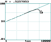
Example #1 (Hurst exponent of brown noise):

-
Example #2 (Hurst exponent of Lorenz
x(t)
data)
 Capacity Dimension
-
The most direct indication of chaos is a strange attractor
-
Strange attractors will generally have a low, non-integer dimension
-
There are many ways to define and calculate the dimension
-
We already encountered the Kaplan-Yorke dimension, but it requires
knowledge of all the Lyapunov exponents
-
Most calculations depend on the fact that amount of "stuff" M scales
as dD where d is the linear size of a "box"
-
Hence D = d log(M) / d log(d) [i.e.,
D
is the slope of log(M) versus log(d)]
-
One example is the capacity dimension (D0)
-
Closely related to the Hausdorff dimension or "cover dimension"
-
Consider data representing a line and a surface embedded
in 2-D
-
The number of squares N of size d required to cover the line
(1-D) is proportional to 1/d
-
The number of squares N of size d required to cover the surface
(2-D) is proportional to 1/d2
-
The number of squares N of size d required to cover a fractal
(dimension D0) is proportional to 1/dD0
-
Hence the fractal dimension is given by D0
= d log(N) / d log(1/d)
-
This is equivalent to D0 = -d log(N)
/ d log(d)
-
Plot log(N) versus log(d) and take the (negative)
slope
to get D0
-
More typically D0 is calculated using a grid of fixed
squares
-
Example (2000 data points from Hénon
map with DE = 2)
-
This derivative should be taken in the limit d --> 0
-
The idea can be generalized to DE > 2 using (hyper)cubes
-
Many data points are required to get a good result
-
The number required increases exponentially with D0
-
If 10 points are needed to define a line (1-D),
then 100 points are needed to define a surface (2-D),
and 1000 points are needed to define a volume (3-D), etc.
 Examples of Fractals
-
There are many other ways to make fractals besides chaotic dynamics
-
They are worthy of study in their own right
-
They provide a new way of viewing the world
-
Fractal slide show (another "lecture within a lecture")
-
Some of these cases will be studied more later in the semester
 Similarity Dimension
-
Easy to calculate dimension for exactly self-similar fractals
-
Example #1 (Sierpinski carpet):
-

-
Consists of 9 squares in a 3 x 3 array
-
Eight squares are self-similar squares and one is empty
-
Each time the linear scale is increased 3 x, the "stuff" increases 8 times
Hence, D = log(8) / log(3) = 1.892789261...
-
Note: Any base can be used for log since it involves a ratio
-
Example #2 (Koch curve):
-

-
Consists of 4 line segments: _/\_
-
Each factor of 3 increase in length adds 4 x the "stuff"
Hence, D = log(4) / log(3) = 1.261859507...
-
Example #3 (Triadic Cantor set):
-

-
Consists of three line segments _____ _____ _____
-
Two segments are self similar and one is empty
-
Each factor of 3 increase in length adds 2 x the "stuff"
-
Hence, D = log(2) / log(3) = 0.630929753
J. C. Sprott | Physics 505
Home Page | Previous Lecture | Next
Lecture


