Henon Map Correlation Dimension

The parameter b is a measure of the rate of area contraction (dissipation), and the Henon map is the most general 2-D quadratic map with the property that the contraction is independent of x and y. For b = 0, the Henon map reduces to the quadratic map, which is conjugate to the logistic map. Bounded solutions exist for the Henon map over a range of a and b values, and a portion of this range (about 6%) yields chaotic solutions as shown below:

The chaotic solutions lie on a beach on the northwest edge of the island of bounded solutions. The usual values used to produce chaotic solutions are a = -1.4, b = 0.3. Initial conditions of x = 0, y = 0 will suffice but lead to a few spurious transient points. Better initial conditions can be chosen near one of the unstable fixed points such as x = 0.63135448, y = 0.18940634. These values yield in the xy-plane the strange attractor with its basin of attraction in black:

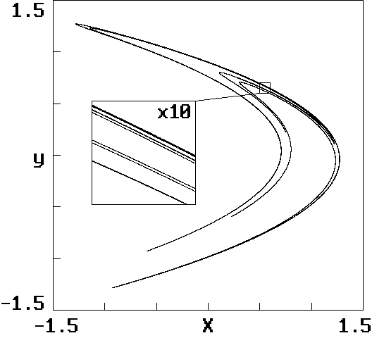
Initial conditions in the white regions outside the basin are attracted to infinity. A more detailed view of the attractor reveals its fractal structure in the 10x magnified insert below:

To calculate the correlation dimension, one would normally generate a time series of some appropriate number of successive x iterates and then, from the separation of every pair of points in xy-space, construct the function C(r) whose logarithmic derivative approximates the correlation dimension. With short data records obtained with difficulty from real-world experiments, this procedure is appropriate. Grassberger and Procaccia used this method with 15,000 data points to estimate a correlation dimension of 1.21±0.01 for the Henon map. However, with numerical data, we usually have the luxury of generating a time series of arbitrary length. The computational cost of producing additional data may be insignificant compared with the cost of computing the correlation dimension.

In such a case, a preferable strategy is to maintain a circular buffer of previous points. Each new iterate replaces the oldest point in the buffer, which is then discarded. As each new point is added to the buffer, its separation from each of the previous points is calculated and sorted into bins. A few of the most recent points are excluded to avoid errors due to temporal correlation. For example, with the Henon map, the largest Lyapunov exponent is known to be about 0.603 bits/iteration, and so after 133 iterations in 80-bit precision, no temporal correlations should remain. Thus the buffer need not be particularly large. For the work reported here, a buffer of 6150 points was used, and the most recent 150 points were ignored. This choice allows the buffer to reside in one 64 K memory block of 10-byte (extended-precision) variables. The computational cost of iterating the map is negligible compared with the cost of performing 6000 correlations.

The accuracy with which a correlation dimension can be calculated is dictated by the number of pairs of data points that are correlated. With abundant data, there is thus a premium on calculating and binning the separations as quickly as possible. The Euclidean separation between two points (x₁, y₁) and (x₂, y₂) is normally calculated from r = [(x₂ - x₁)² + (y₂ - y₁)²]^1/2. It has been proposed to use other measures such as the absolute norm, r = |x₂ - x₁| + |y₂ - y₁|, or the maximum norm, r = max[|x₂ - x₁|, |y₂ - y₁|], but these methods tend to give inferior results. Note, however, that it is not necessary to perform the square root; it is just as good to bin the values of r² as it is to bin the values of r.

With bins of width dr proportional to r, there are several strategies for sorting the separations into the appropriate bin. The conceptually simplest method is to generate a bin index by taking the integer part of c log(r²), where c is a constant chosen to give the desired bin width. Calculation of the logarithm typically limits the speed of this method. An alternate method is to start with a large reference value of R² and divide it repeatedly by a constant factor c until it is less than r². A count of the number of divisions then gives a bin index. This method is reasonably fast if the bin width (c) is large.

A clever scheme is to make use of the fact that computers store floating point numbers with a mantissa and integer exponent of 2. Thus it is possible to find the integer part of log₂(r²) by extracting the appropriate bits of the variable r². A Microsoft BASIC expression that returns the integer part of log₂(A) where A is a double-precision (8-byte) variable in IEEE format is 16 * PEEK(VARPTR(A) + 7) + PEEK(VARPTR(A) + 6) \ 16 - 1023. This statement executes significantly faster than the equivalent BASIC statement INT(1.442695041 * LOG(A)). This method automatically gives 2 / log₁₀(2) = 6.64 bins per decade if A = r², which is reasonable for many cases. To double the number of bins, it is only necessary to use A = r⁴, which requires one additional multiplication. In this note, we use A = r¹⁶, which gives 16 / log₁₀(2) = 53.15 bins per decade.

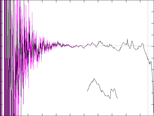
The short wiggly line toward the bottom is a portion of the upper curve magnified by a factor of 16 (see ZOOM.DAT). It appears that the plot of D(r) may itself be a fractal with at least statistical self-similarity. The calculation of the correlation dimension assumes that D(r) approaches a limiting value as r --> 0. It is not obvious whether this is the case. The variations in D do seem to decrease as r decreases, at least until the statistical errors dominate, but the convergence is very slow. The calculations are still being refined to clarify this issue.